Definite integrals and their applications
The app computes a definite integral by the Newton–Leibniz formula (the fundamental theorem of calculus) and draws the area under the graph – the part above the x-axis in a different colour from the part below. It also handles improper integrals and applications: area, arc length, volume and surface area of a solid of revolution, also for curves given parametrically and in polar coordinates.
Definite integral
The app finds the antiderivative as for an indefinite integral and substitutes the limits. With a substitution it converts the limits right away. If the integral has no elementary antiderivative, it computes it numerically.
How to enter it
int(x^2, x, 0, 3) | An integral with the variable and the limits. |
\int_{0}^{\pi} \sin x\,dx | From a photo or in LaTeX. |
x^2 | A function with the “Integrate” chip – fill in the limits in the fields. |
Examples
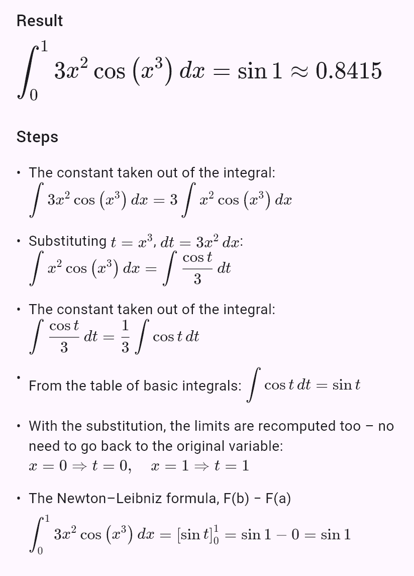
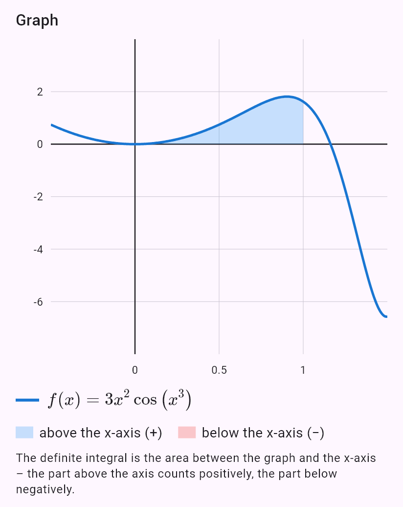
int(3x^2 cos(x^3), x, 0, 1)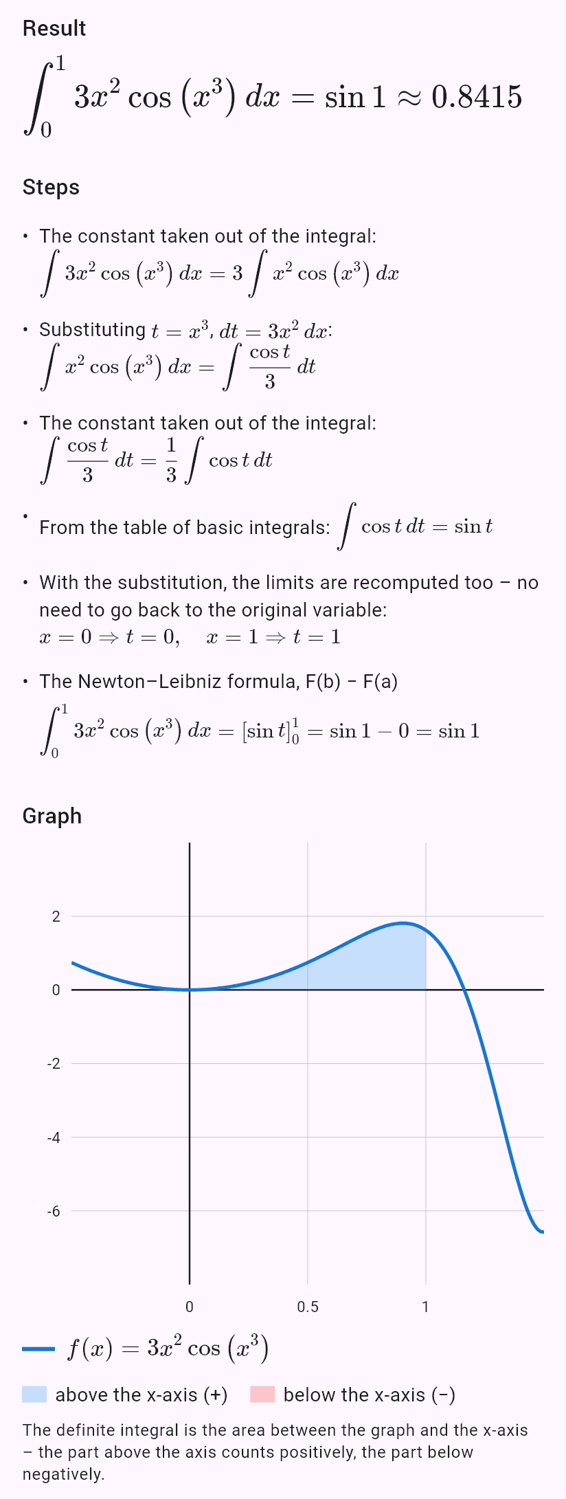
Improper integrals
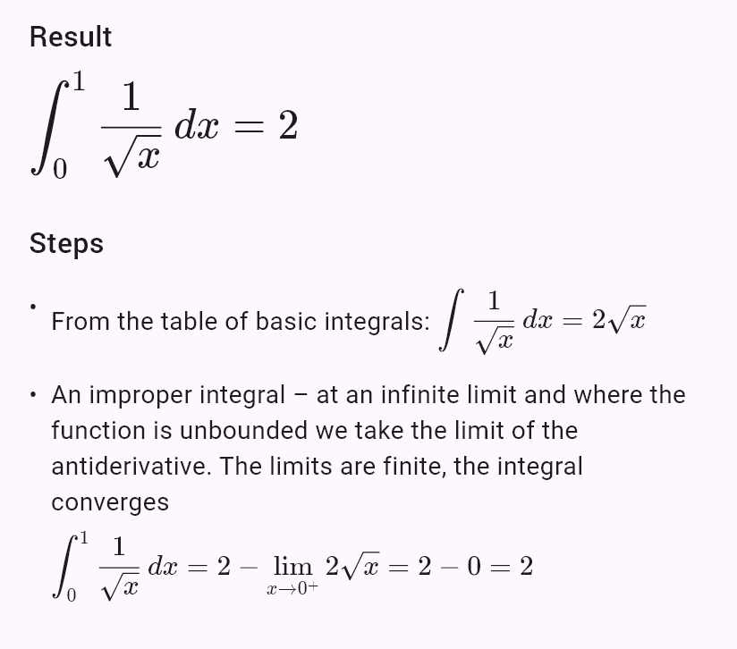
The app handles an infinite limit or an unbounded function with a limit of the antiderivative and says whether the integral converges or diverges. If that limit cannot be computed, it decides by a comparison test.
Examples
int(1/x^2, x, 1, oo)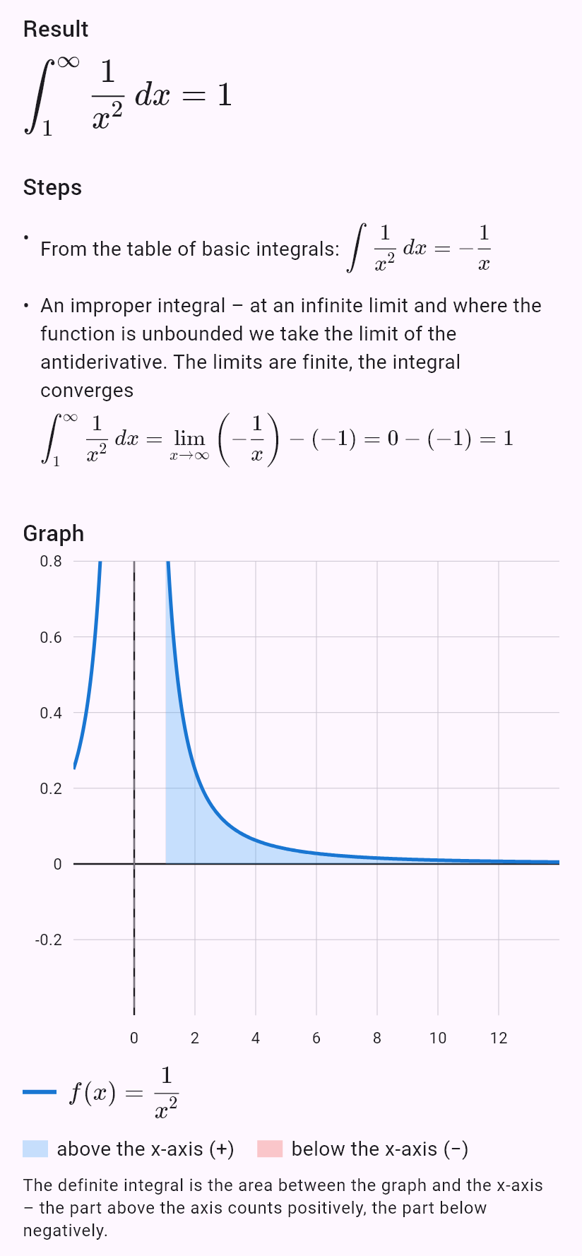
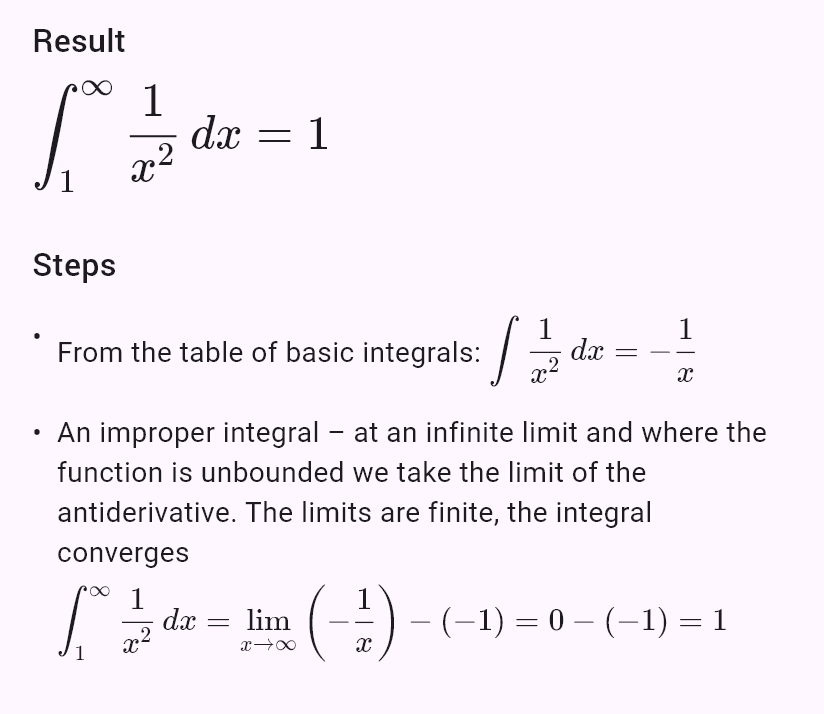
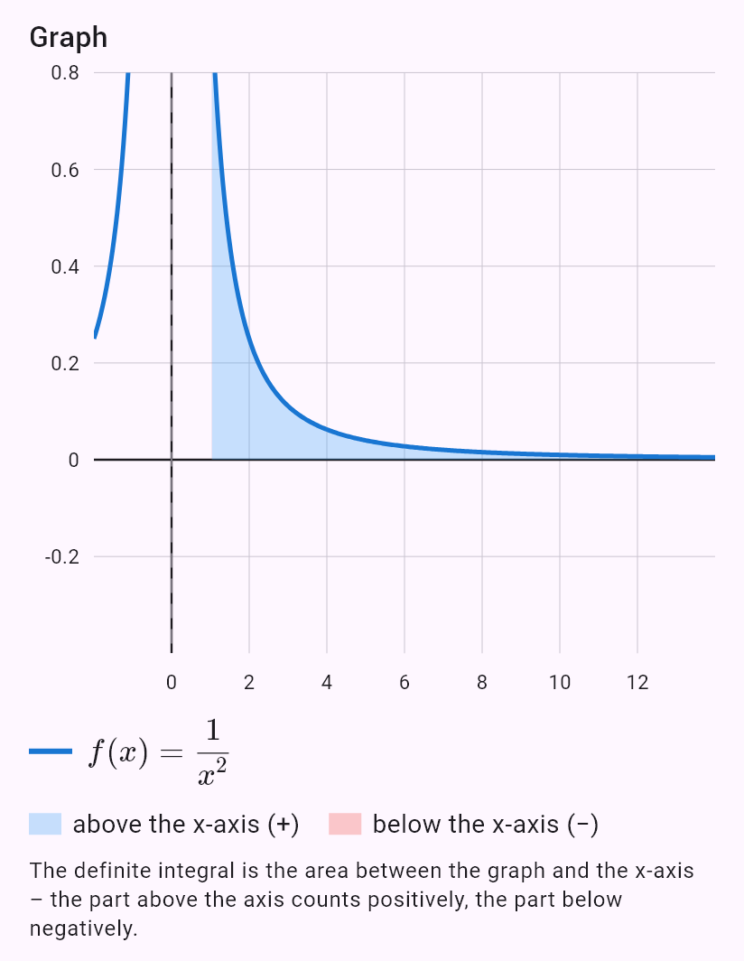
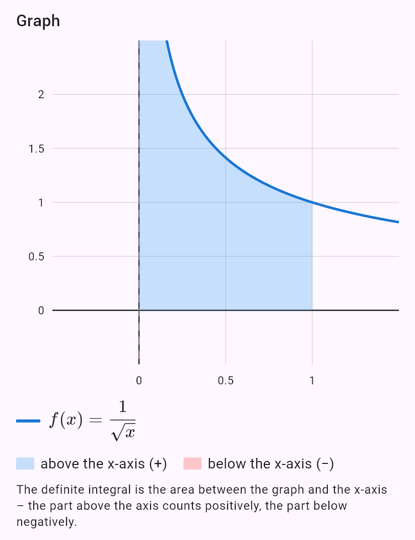
int(1/sqrt(x), x, 0, 1)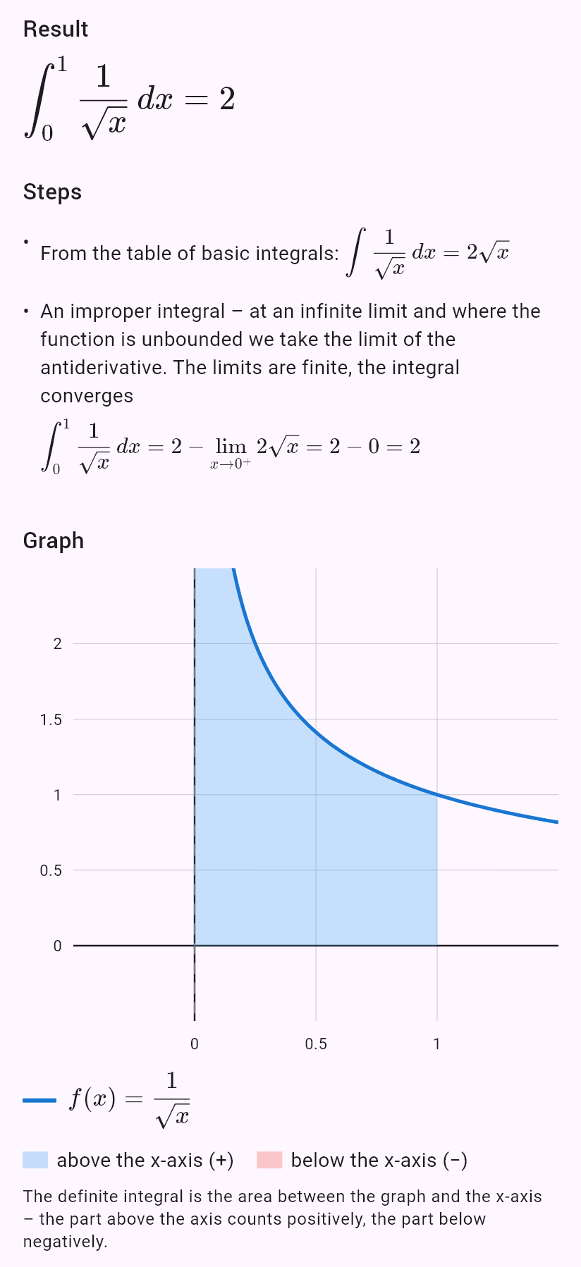
Area under a curve and between curves
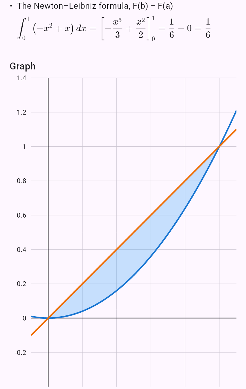
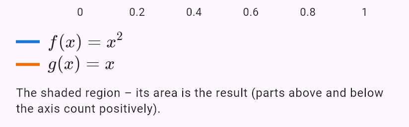
The app computes the area between a graph and the x-axis, or between two curves, as the integral of the absolute value of the difference – parts above and below both count as positive. You don't have to enter the limits: it finds them as the intersections of the curves.
How to enter it
area(x^2, x) | The area between two curves, limits from the intersections. |
area(sin x, 0, pi) | The area between a curve and the x-axis on an interval. |
x^2 | A function with the “Integrate” chip → “Area between curves”; fill in the second curve and the limits in the fields. |
Examples
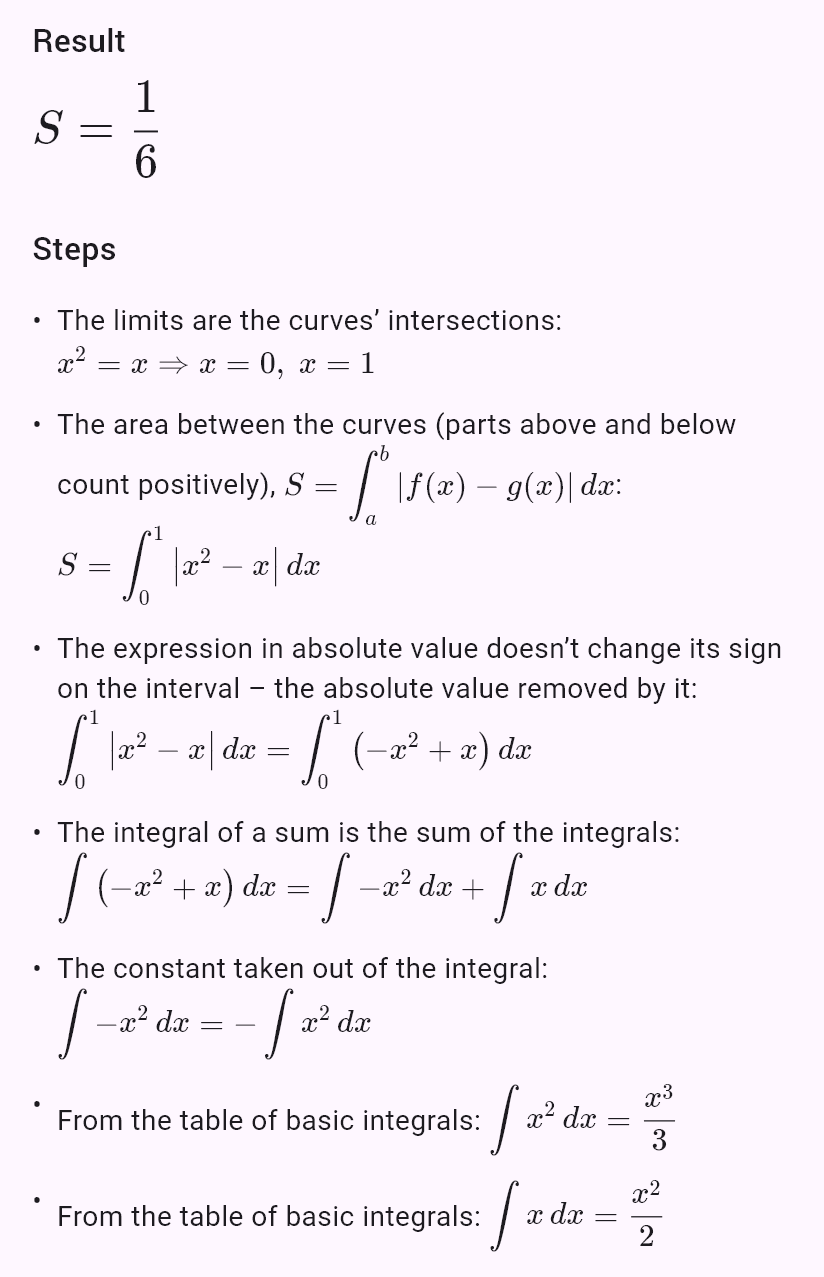
x^2 Area between curves, second curve x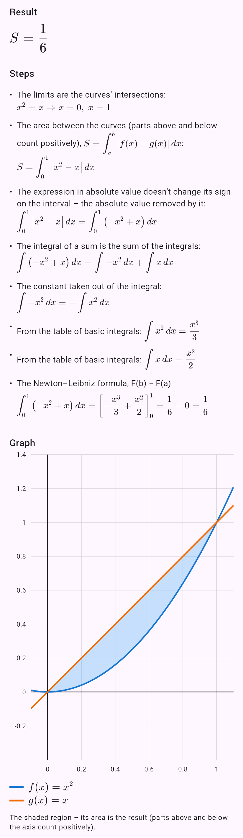
Arc length
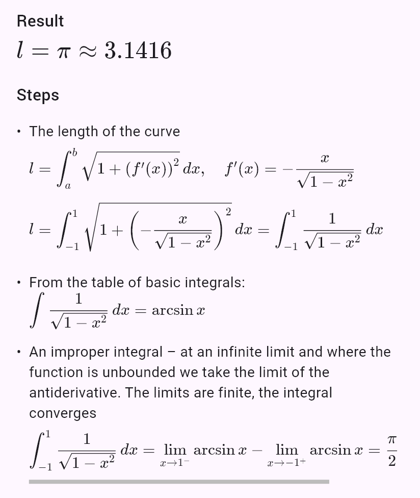
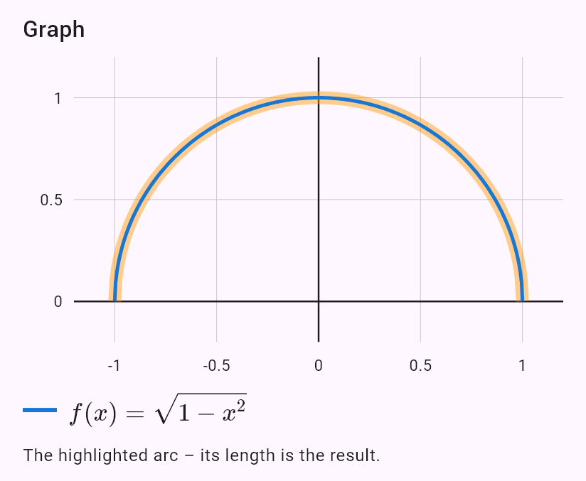
The app computes the length of a graph on an interval by the formula l = ∫√(1 + f′²) dx. It tries to simplify the root (for a semicircle it comes out as arcsine); where the integral has no elementary antiderivative, the result is numerical.
How to enter it
length(x^(3/2), 0, 4) | The arc length on an interval. |
Examples
sqrt(1 - x^2) Arc length, limits −1 and 1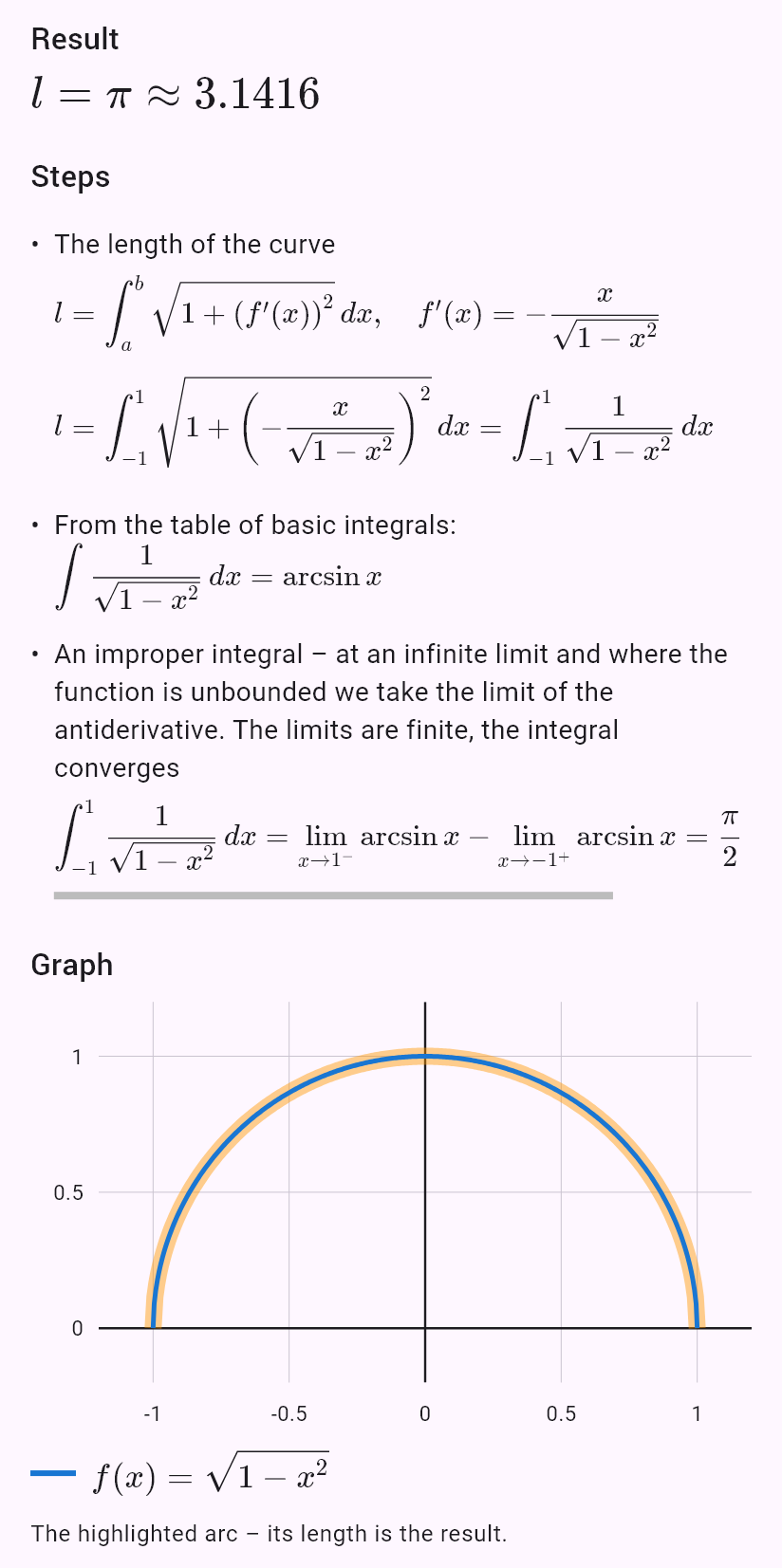
Volume of a solid of revolution
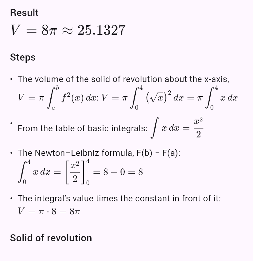
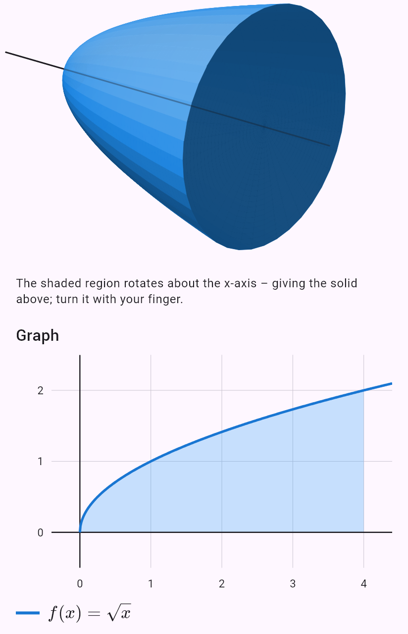
The app computes the volume of a solid of revolution about the x-axis by the formula V = π∫f² dx (between two curves as washers), about the y-axis by the shell method. It also shows the solid in 3D – rotate it with your finger.
How to enter it
volume(sqrt(x), 0, 4) | The volume of the solid rotated about the x-axis. |
volume(x^2, 0, 2, y) | Rotation about the y-axis. |
Examples
sqrt(x) Volume of a solid, limits 0 and 4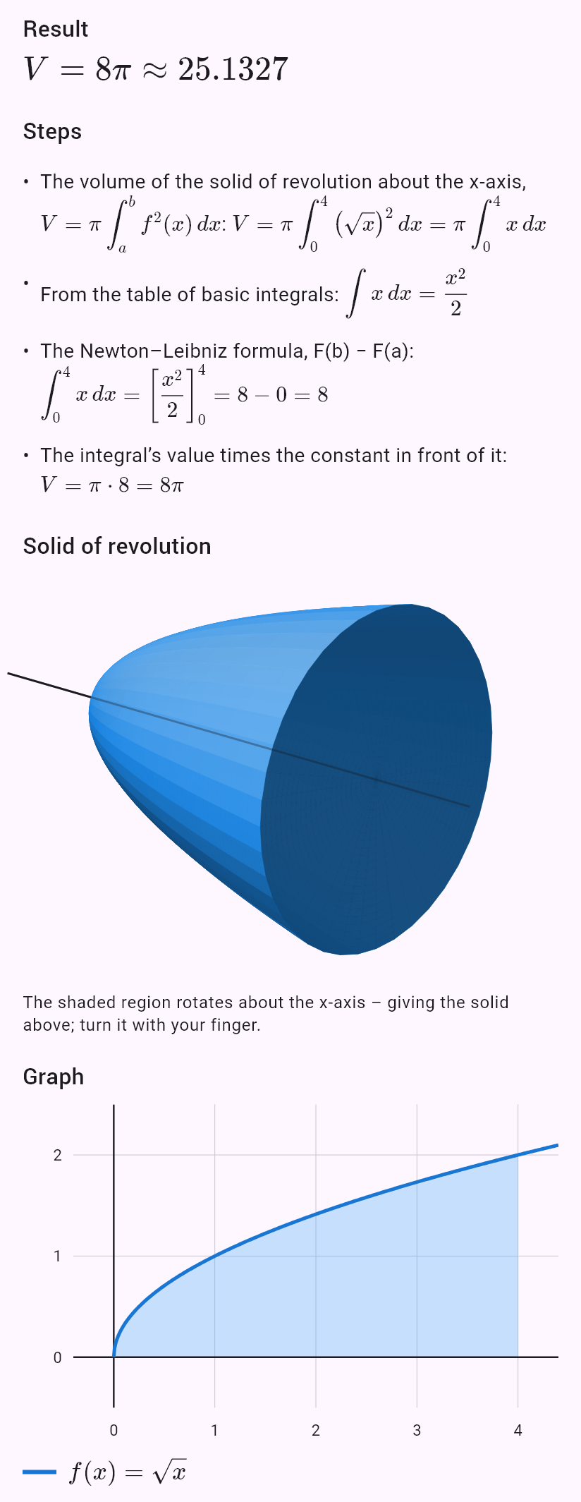
Surface area of a solid of revolution
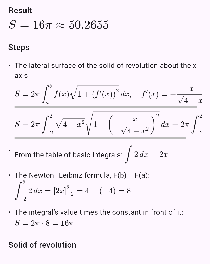
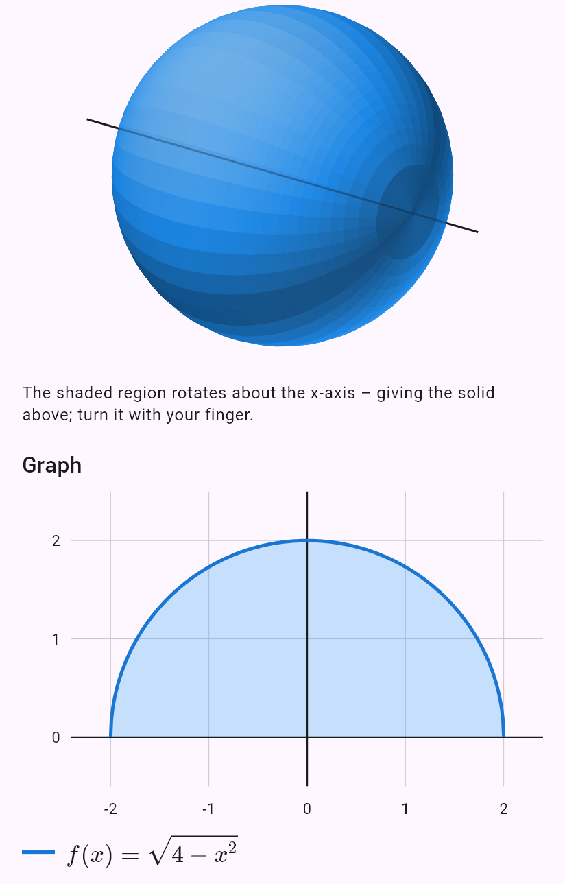
The app computes the lateral surface area by the formula S = 2π∫f√(1 + f′²) dx; the product under the root often simplifies (for a sphere it comes out constant).
How to enter it
surface(sqrt(4 - x^2), -2, 2) | The surface of the solid rotated about the x-axis. |
Examples
sqrt(4 - x^2) Surface of a solid, limits −2 and 2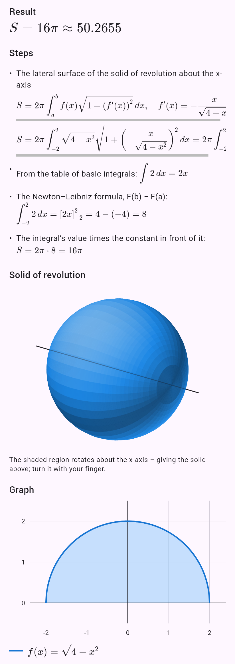
Parametric curves and curves in polar coordinates
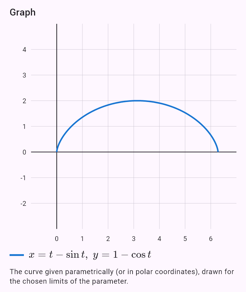
Write a curve x = φ(t), y = ψ(t) on two lines, a curve in polar coordinates as r = ρ(φ). The “Integrate” chip then offers the area, length, volume and surface; the limits of the parameter are optional (without them from 0 to 2π). Volume and surface are computed by rotating the part of the curve above the x-axis about the x-axis.
How to enter it
x = t - sin(t) | A parametric curve on two lines. |
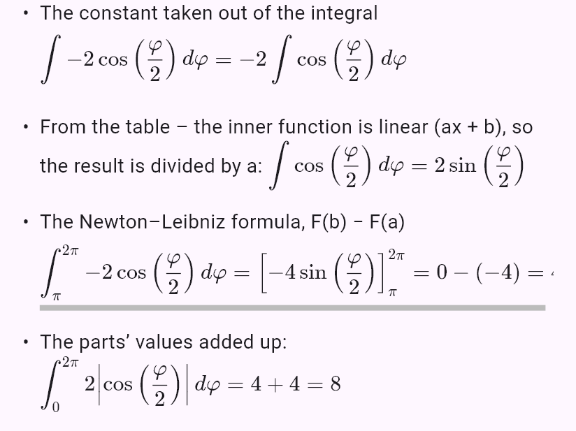
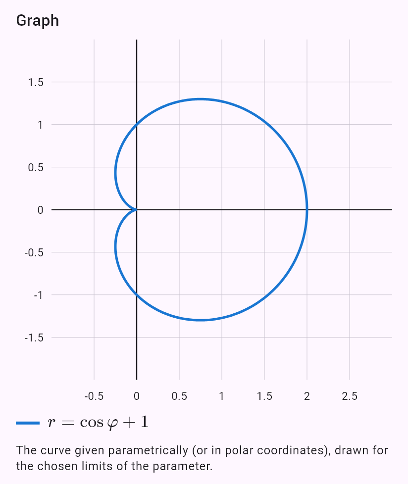
r = 1 + cos(phi) | A curve in polar coordinates (also r^2 = … for a lemniscate). |
length(x=cos(t)^3, y=sin(t)^3, t, 0, 2pi) | The written form with the parameter and the limits. |
Examples
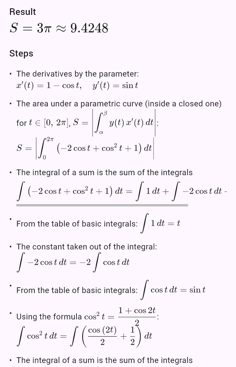
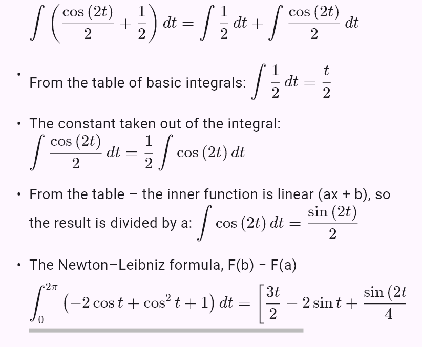
x = t - sin(t)
y = 1 - cos(t) Area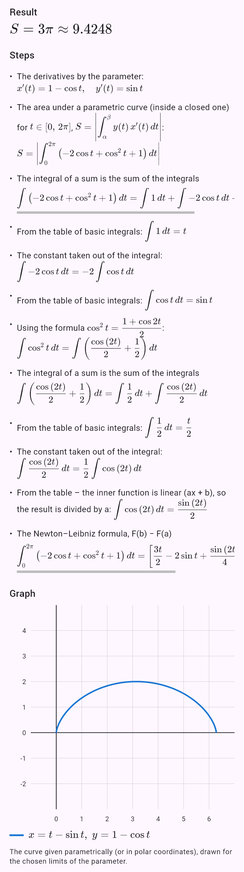
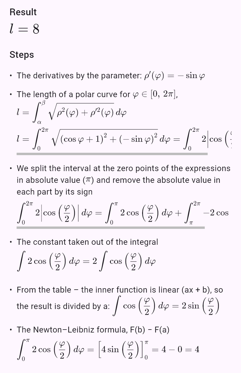
r = 1 + cos(phi) Arc length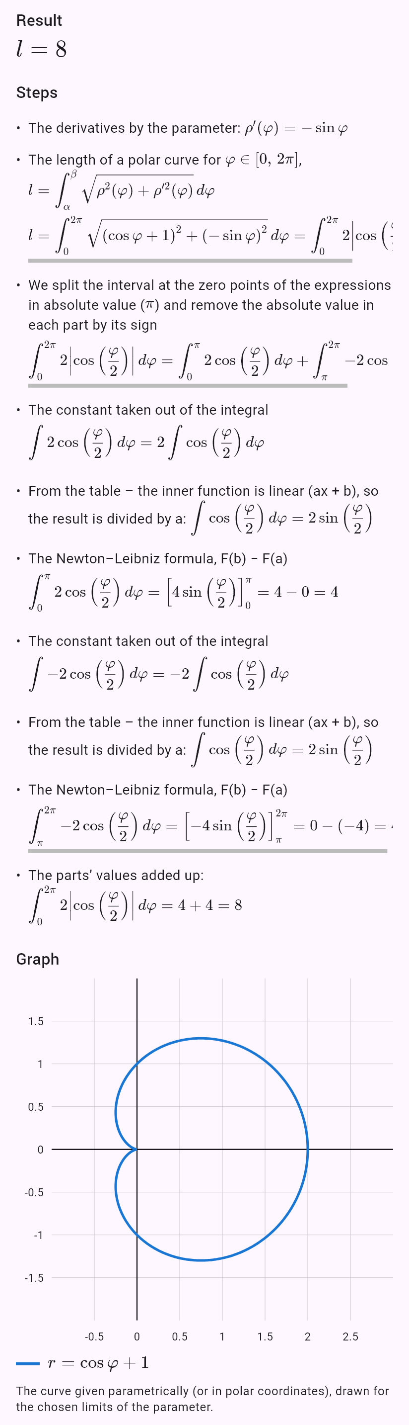
Curves given by an equation
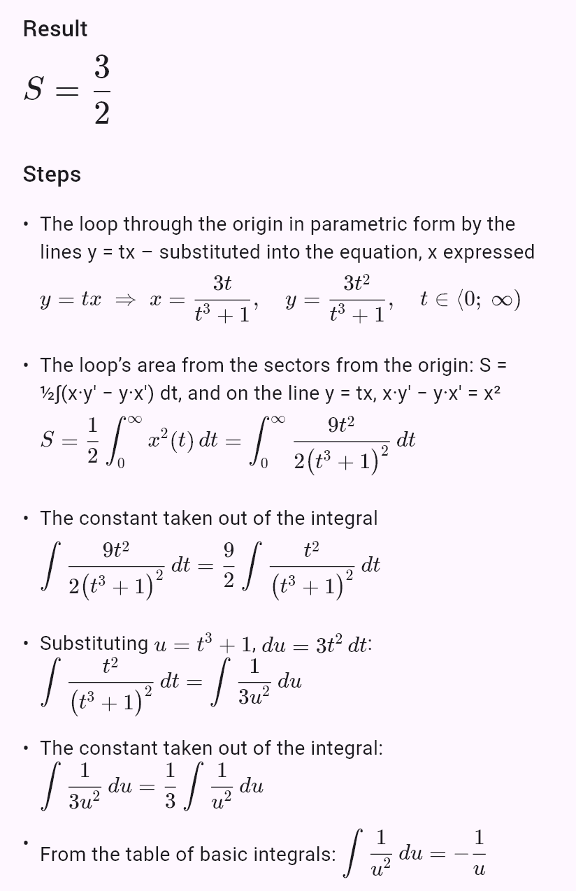
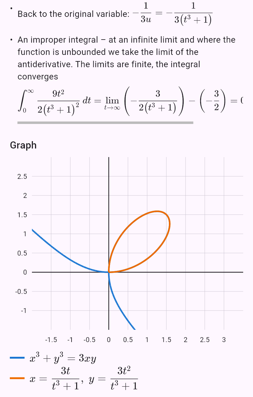
For an equation in x and y (x³ + y³ = 3xy) the “Integrate” chip offers the area, the length, the volume and the surface. Without limits it takes the whole closed curve: a circle or an ellipse in parametric form by cos and sin, a loop through the origin (the folium of Descartes) by the lines y = tx – the loop’s area then exactly from the sectors, the length, volume and surface numerically. With limits in x it uses the upper branch y = f(x).
How to enter it
x^3 + y^3 = 3xy | A closed curve – the “Integrate” chip without limits. |
y^2 = x^3 | A curve that isn’t closed – the “Integrate” chip with limits in x (the upper branch y = x^(3/2)). |
Examples
x^3 + y^3 = 3xy Integrate → Area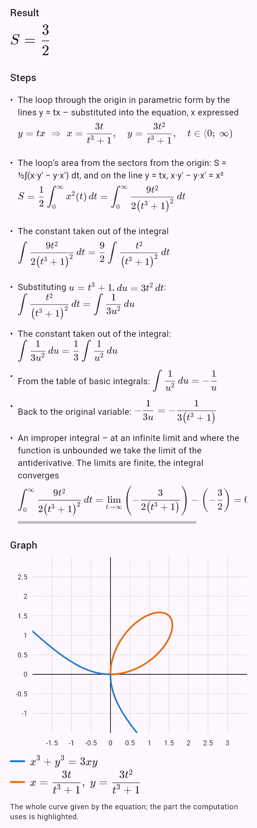

Known limitations
- The arc length of y = ∛x (and similar curves) is only computed numerically – it leads to an elliptic integral, which has no elementary antiderivative.
- For parametric and polar curves the shaded area and the 3D solid are still missing; rotation only about the x-axis.
- Rotation about the y-axis only for a region on one side of the axis.
- For implicit curves without limits only a circle, an ellipse and a loop through the origin are supported; rotation only about the x-axis.